How to identify a customer’s nearest store by drive-time

8 min read

Discover some practical examples outlining our latest improvements to drive-time calculations.

Introduction

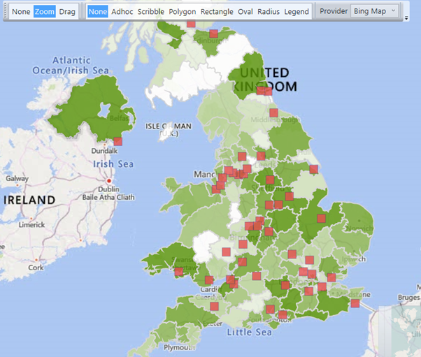
Many marketing analysts will have lots of locations of interest (such as airports for travel firms, retail stores, tourist attractions etc). Understanding customers proximity to these locations, or being able to action marketing campaigns based on metrics related to them can be a vital activity. In this blog post, we will illustrate these ideas with relation to a company who have 46 retail stores located across the United Kingdom (Note 1). We can see the distribution of these stores in the map below, where I have a thematic map of the volumes of my customers by postal area, and the store locations highlighted as red squares.

In 2018, I wrote a blog post called ‘Geographic Expressions in FastStats’. In it, I showed some straight-line distance expression functions and how they could be used for finding nearest locations and the distance to nearest location as the crow flies. These expressions can be useful, but have a big weakness. 

If the geography of the real-world means that straight-line distance is an impractical measure (e.g. mountains/water get in the way), then these expressions are less useful to the marketer. For example, invitations to an event based on location is less relevant if a customer cannot travel to that location very easily.

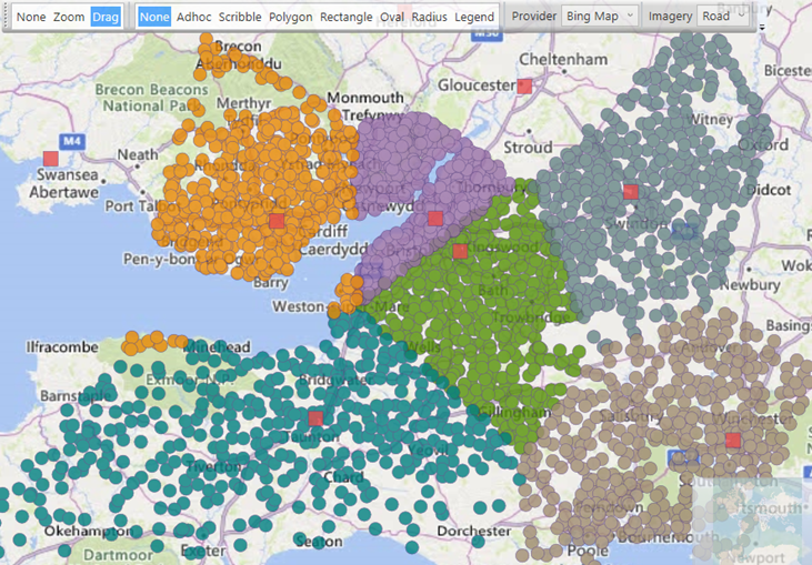
We can see that neatly in the example below. The orange dots represent customers whose nearest direct line store is Cardiff, yet there are two pockets (around Weston Super Mare and Lynmouth) where the shortest straight-line distance to a store is going to require some swimming! If we were to action a marketing campaign to those customers based on visiting that store, it is unlikely to be effective!

In this blog post, we will showcase some recent mapping developments, which will help us overcome this problem, and provide the ability to analyse our customers by a range of different metrics. 

Travel-time analysis

The obvious proximity measures for a relevant location (e.g. a store, airport etc) is knowing how long it takes each customer to travel to that location. For different types of business, the size of the driving catchment area will be different – I’d drive further to go to the airport for my annual holiday than I would to visit the cinema for example. In some instances, the mode of transport will also be different – for instance, for a coffee shop it may be that walking time is a critical metric.

FastStats has long offered the ability to do drive-time calculations, but there have been trade-offs that the analyst has had to make. In the DriveZone wizard, the drive zones are matched to an underlying geographical shape file (e.g. postal district) which leads to a level of inaccuracy proportional to the size of the shape files. In the Point to Point wizard, the drive-times are calculated exactly for every customer location to the point of interest. This is an intensive time-consuming process that renders it suitable only for a limited number of records. Alternatively, drive-times are again calculated to a bigger area such as postal district to enable more records to be classified, at the expense of accuracy in the calculations.

However, our recent developments in these wizards have enabled the DriveZone wizard to match to drive zones exactly, and the Point to Point wizard can much more efficiently categorise records into numerical drive-time values.

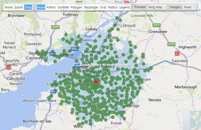
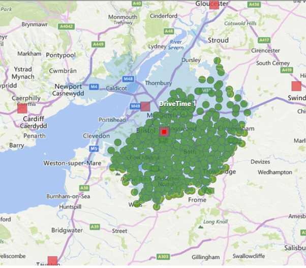
In my retail example, I believe that given the size of the stores, that say 40 minutes is a maximum drive-time that someone would undertake to visit one of these stores. In the screenshot below, I have constructed a 40-minute drive-time zone around the Bristol South store, and then plotted some of the customers who live within that catchment area. We can see that there are a number who live in South Wales, and that we can go further down the arterial M4/M5 motorways than in other directions. 

We could use such a selection to target people who live within that drive-time of this store, but there are a number of them who are much more likely to go a different store, because there is a closer alternative (Cardiff, Gloucester, Bristol North or Swindon for example).  

It is much more powerful and useful for us to be able to identify a customer’s nearest store by drive-time.

Nearest location by drive-time

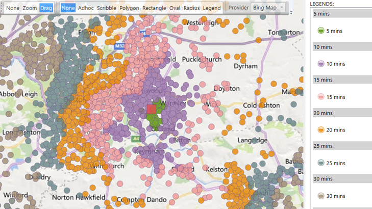
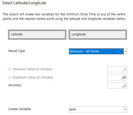
In the Q3 2022 release, we have introduced a new section to the Point to Point wizard which will allow for a range of different drive-time analysis tasks. The first and most obvious one is to provide drive-time between a location of interest and each customer record in a much more efficient process than previously. The user can specify a maximum drive-time of interest, and how accurately they want to calculate the drive-time between these values. In the screenshot below, I am working out the drive-time in minutes between 0-80 to an accuracy of 5 minutes (i.e those in 5/10/15/20/25/30/35/40/45/50/55/60/65/70/75/80 minutes, with different colour dots radiating outwards) from the Bristol South store. The reasoning here is that I don’t need to work out the number more accurately than this, as a 5-minute difference probably won’t affect whether a customer may travel to one location or another.

We can go so much further now with this line of thinking. Being able to identify the customers nearest store by drive-time is hugely powerful, but would previously have taken a lot of manual work to achieve, whereas now you can simply ask for it in the wizard, as in the screenshot below.

Furthermore, this result is now returned in much quicker time than it would have done previously. If we change our previous example to select customers for whom Bristol South is their nearest store, we get a different picture. I have left the 40-minute drive-time on the map, so we can see the resulting effect more clearly in the screenshot below. Customers to the South East of Bristol remain selected, but all those in South Wales and Gloucestershire will have been allocated to the Cardiff, Bristol North or Gloucester stores respectively. This is a much improved targeted selection and we are focusing on the relevant customers more accurately.

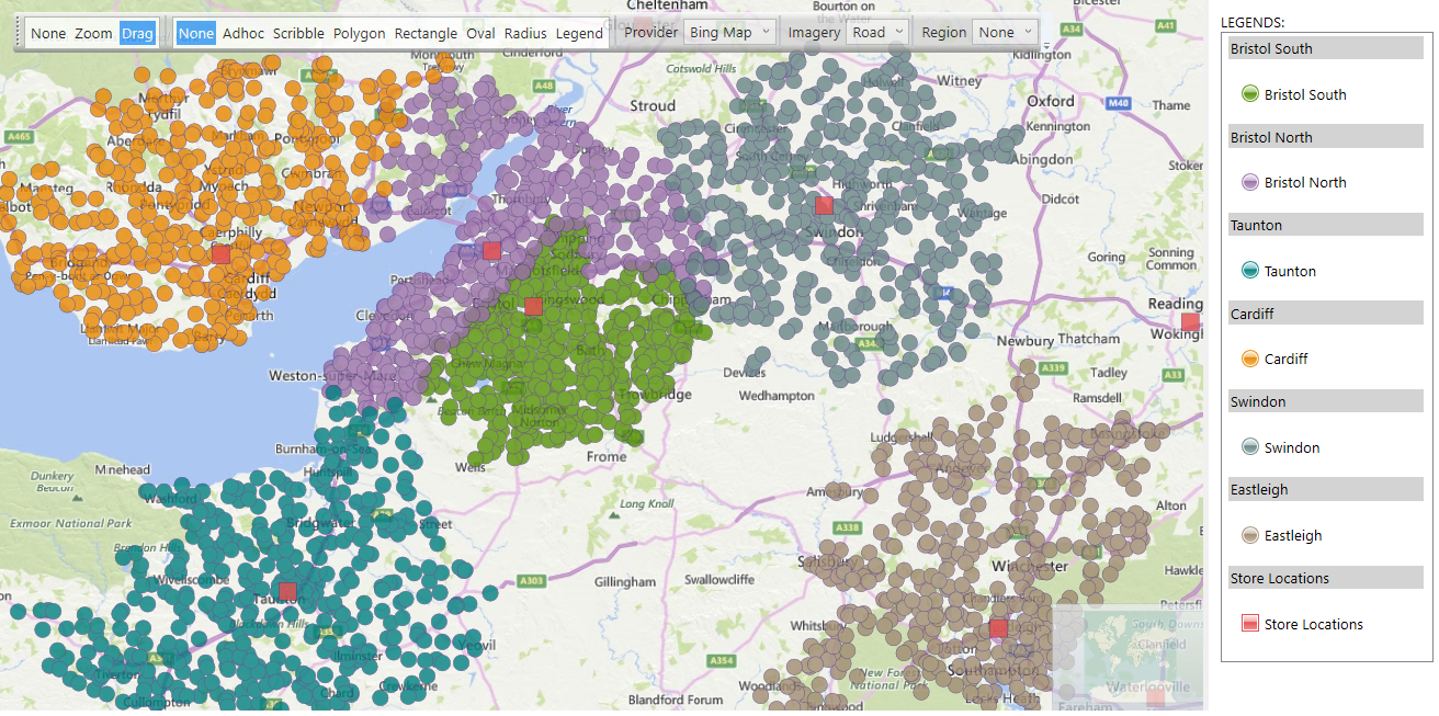
The next screenshot embellishes the above one slightly – we have now highlighted several groups who can reach their nearest store in 40 minutes, and plotted them by their nearest stores (Cardiff, Taunton, Bristol North, Swindon and Eastleigh). We can see the boundary between the two Bristol stores and the Swindon store nicely in this example. Furthermore, there is a large gap in Somerset/Dorset where customers would take over 40 minutes to get to any of the stores.

In some instances, we might also be interested in the 2nd/3rd etc nearest locations, so this option is also supported if you wanted to send out communications with a number of possible locations or stores for the customer to visit.

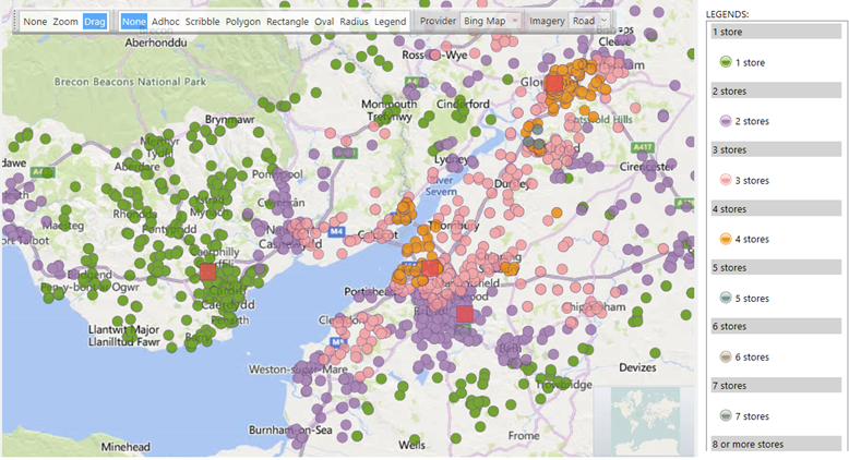
In some scenarios, the number of points of interest that are within X minutes drive-time may be important. For example, with respect to customer retention and engagement – if these are visitor attractions, hotels, etc then customers may be more engaged if there are a larger number of them within easy driving time of their home. We can support this scenario as a simple numeric metric using the wizard, where the user simply has to choose the minimum and/or maximum drive-times to count the points within. In the example below, we have coloured different customers by the number of stores they can reach within 1 hour. There is a small cluster of people around the Severn crossing, who can reach four stores within 40 minutes-drive. There are also other customers around Gloucester who can also reach four stores. Further North, there is an area between Manchester and Liverpool where customers could reach at least eight stores within 40 minutes- drive!

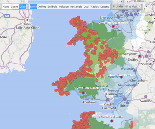
This technique can also be used to conversely find areas where there are 0 locations a customer can reach easily. In the screenshot below, I have plotted customers who cannot reach any store in 40 minutes, and I have overlaid a number of drive-time zones from stores that show that these customers have travelled longer times to get to one of our locations. We can see the big gaps in West Wales, and in Somerset/Dorset as per our previous screenshot. 

Conclusion

These developments in the Q3 2022 version of the Apteco marketing software make it much more realistic for analysts to be able to carry out drive-time based analysis on larger numbers of records than previously possible, and allow for new insights to be derived, and for those to drive more targeted marketing campaigns.

References
Note 1 – These 46 locations are actually the exact locations of the larger stores of a prominent UK retailer who have an interesting geographic dispersion of store locations across the whole of the UK. I have not identified this company by name in the blog!