On-the-fly Aggregations part 3
27 Nov 2018 | by Chris Roe
We introduce a new type of aggregation and demonstrate how it can provide deeper data analysis.
Introduction
In the Q4 2017 release we introduced the ‘on-the-fly aggregation’ capabilities and published two introductory blog posts on this (which you can find here and here). In this blog post we’re going to delve a bit deeper into this functionality.
- Firstly, we’ll show a new type of aggregation (MaxCategory).
- Secondly, we’ll show how the general functionality can be used recursively to answer more complicated questions whilst avoiding the need to create intermediate virtual variables.
- In the final section, we’ll show some examples of segmentation selections that use on-the-fly aggregations within expressions to also extend the capabilities in this area.
MaxCategory
Which destination have my customers spent most on?
Which product do they buy the most?
Which communication channel is preferred by this customer?
All of these questions could have been answered previously using FastStats, but this extension to the on-the-fly aggregation functionality makes it much quicker to create and maintain objects that seek to answer them.
Prior to Q4 2017, a virtual variable would have had to be created for each product grouping. This may have been acceptable when you have three products, but as the number of products increases it becomes a pain – quickly followed by too much hassle. Before the MaxCategory aggregations this could have been achieved by using an on-the-fly aggregation for each of the product groupings and a much more complicated expression. Now this can be achieved with a single on-the-fly aggregation.
Let’s look at an example of how to specify an on-the-fly aggregation using our fictitious holiday company FastStats system to answer the first of the questions posed above.
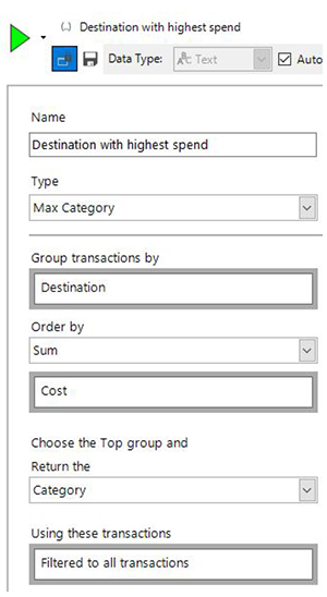
Here we start by taking the transactions for each person and grouping them by the Destination variable into a number of sets. We then work out the Sum(Cost) for each of those sets and find the one with the highest value.
There are a number of different ways of ordering the resulting groups. We’re then able to choose which function to apply to the resulting best set in order to return a value. Some of them are numeric (such as working out the amount I’ve spent on my highest value destination). The one in the example above is categorical – it will return the name of the destination.
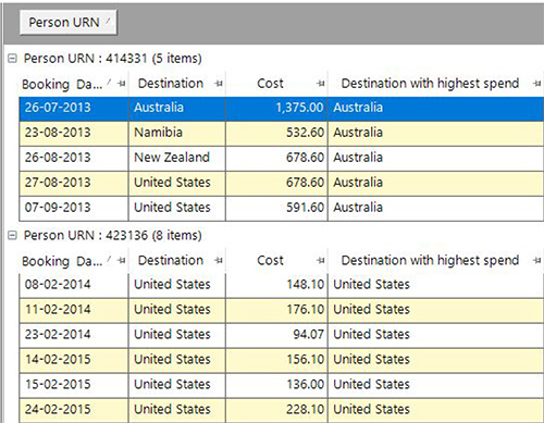
We can check the results of this aggregation by adding the expression to a data grid. In the example of the top person, the sum of their one transaction to Australia is greater than the sum of their two to the USA.
We’ll be looking to extend this to allow a wider range of functions and the ability to pick not just the top group – although this is the one that will have the most common use case in marketing analytics. The above aggregation can be used on its own within an expression or combined in an expression in any way you wish. For example, you may want to find out whether the highest value destination this year is the same as last year for each customer. There are so many possibilities!
Multi-level aggregations
How many transactions did a customer make in the year after their first transaction? This can be a useful attribute to analyse or use in a predictive model. Prior to the on-the-fly aggregation functionality this would have been a more long-winded process.
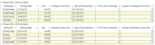
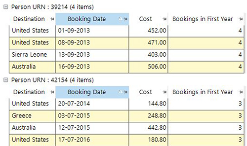
Firstly, we would need to create a virtual variable to record the first transaction date for a customer and store that as a date variable (see column Date of First Booking below).
Secondly, we would need to create an expression to flag all records where the transaction date of that record was within one year of the variable we created in the first step (see In First Year of Booking column below). We could then use this as an attribute to apply the RFV selection to, or as a transactional selection within a further frequency virtual variable to create the required value as a variable (see Number of Bookings in First Year column).
We can use the on-the-fly aggregation functionality to work out all the steps below without having to create any virtual variables at all. The approach is similar to above.
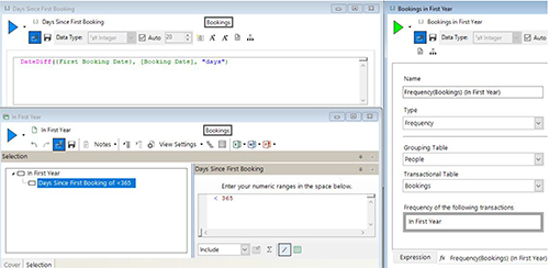
The screenshot below shows the required steps. We start in the top left by creating an expression to work out the difference between the first booking date and the current booking date for all bookings.
The first booking date is specified as an on-the-fly recency aggregation. In the bottom right we can then use this expression in a selection to select all bookings where this value is <365 (i.e falls in the first year). We can then use that in a further expression as the transactional filter selection on a frequency aggregation to work out the number of bookings in the first year.
In the example below we’ve added this expression to a data grid to check that the results look correct.
This is a very powerful and flexible technique to extend the capabilities of the on-the-fly aggregation with many possible applications. It could also be used for looking at the ratios of the number of bookings in each year of a customer journey, to see how often a customer switches between products, or to compare how the trend of a customer spend changes between the first half of their transactions and the second.
Segmentations
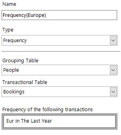
We’ve been unable to formulate up segmentation selections to answer questions for some scenarios as we needed the ability to have aggregations with transactional filter selections containing relative date sliding windows. In the example below we have the definition of a simple Frequency aggregation with a transactional filter to only include bookings made to Europe in the last year.
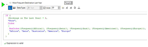
This is just one of several frequency aggregations that we’ve included within the below to try and find out which continent each person has had the most bookings to in the last year. If they’ve not had any bookings then we give them a value of None.
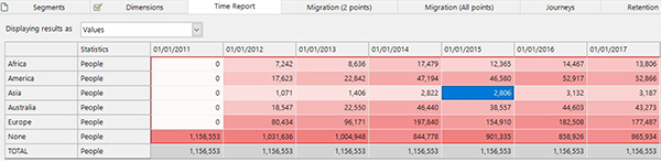
We then create selections based on the above expression for the six possibilities and use those as the definitions of our segments. For each time point within the Segmentation time report the filter selections are translated to ‘The Last Year’ based upon the reporting point. In the report below, the highlighted figure of 2,806 are the customers who had more holidays to Asia than any other continent in the year prior to 01/01/2015 (i.e in 2014) (1).
This kind of approach allows a lot of flexibility for defining complex segmentation selection rules that use a number of on-the-fly aggregations. Other examples of use could be in establishing that a customer had two transactions in the last 60 days and that there was a maximum of 30 days between them.
Conclusions
We can see that there are more in-depth uses of the on-the-fly aggregation functionality introduced in the Q4 2017 release. These extensions add another layer of power and flexibility to their usage within both the expression and segmentation tools.
References
(1) In this example I’ve not been concerned with what happens if someone has had the same number of holidays to multiple continents. In this case, the first occurring continent in the segment list would be chosen first. I deliberately ordered my segments based on an ascending number of total transactions ever to each of these continents to prioritise continents with smaller number of visitors. In many marketing cases you may not be that concerned about which of the equally popular segments you ended up marketing to.